Dithering algorithms compared: Floyd–Steinberg to blue noise
16 dithering algorithms compared on tone, texture, speed and artifacts, with kernels and one table. Which to use for screens, pixel art, lasers and pens.
Updated
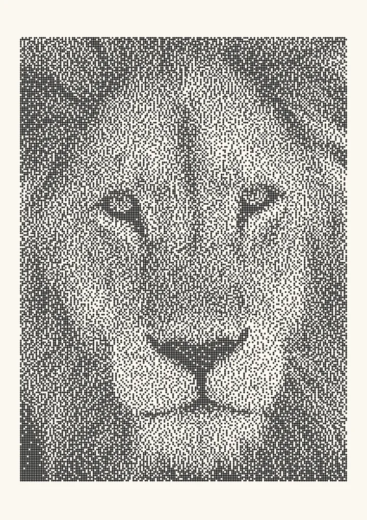

Sample render. Slide to compare the photo with the result. Try the algorithm live below.
Rendered in 0.0 ms on your machine. Every dot here is what a pen or laser would put down.
There are three kinds of dithering algorithm: threshold, ordered and error diffusion. For photographs, use Floyd–Steinberg or Ostromoukhov. For animation, pixel art and anything on a GPU, use Bayer or blue noise. For pens and lasers, use blue noise or Ostromoukhov in linear light. Everything else on this page is the detail behind those three sentences, with the numbers that let you pick for yourself.
You can see every algorithm below on one image on the compare page, and each has its own page with a live demo.
The three families
Threshold compares each pixel to a constant. It is not dithering, but it is the baseline every algorithm is measured against.
Ordered dithering compares each pixel to a value from a tiled pattern. The pattern decides the texture; the pixel decides nothing about its neighbours. One comparison per pixel, fully parallel, identical output every run.
Error diffusion quantises a pixel, then pushes the rounding error onto pixels not yet visited. The kernel (which neighbours, what weights) decides the texture. Sequential by nature, and the output depends on scan order.
Every algorithm in one table
Tone levels for ordered dithers are the number of distinguishable greys the pattern can produce (n² + 1 for an n×n Bayer matrix). “Neighbours” is the number of pixels an error-diffusion kernel writes to. Speed is relative to Floyd–Steinberg on the same image.
| Algorithm | Family | Source | Neighbours / matrix | Divisor | Texture | Main artifact | Speed | Best for |
|---|---|---|---|---|---|---|---|---|
| Threshold | Threshold | – | 1×1 | – | None | Loses all mid-tones | 3× | Stencils, logos |
| Bayer 2×2 | Ordered | Bayer 1973 | 2×2, 5 tones | – | Coarse grid | Only 5 greys | 3× | Chunky retro look |
| Bayer 4×4 | Ordered | Bayer 1973 | 4×4, 17 tones | – | Grid | Crosshatch | 3× | Pixel art, sprites |
| Bayer 8×8 | Ordered | Bayer 1973 | 8×8, 65 tones | – | Fine grid | Crosshatch, banding in 8-bit | 3× | Retro games, GPUs |
| Bayer 16×16 | Ordered | Bayer 1973 | 16×16, 257 tones | – | Very fine grid | Grid still visible | 3× | Large prints with a retro look |
| Blue noise | Ordered | Ulichney 1993 | 128×128 mask | – | Even grain | Slight graininess | 3× | Animation, e-ink, plotters, lasers |
| Floyd–Steinberg | Diffusion | Floyd & Steinberg 1976 | 4 | 16 | Fine, organic | Worms, patches at 1/2, 1/3, 1/4 | 1× | Photos, GIF |
| Atkinson | Diffusion | Bill Atkinson, Apple, 1980s | 6 (only 3/4 of error) | 8 | Crisp, high contrast | Blown highlights and shadows | 1× | Retro Mac look, fast plots |
| Jarvis–Judice–Ninke | Diffusion | JJN 1976 | 12 | 48 | Smooth, soft | Blur, slow | 0.4× | Photos on lasers |
| Stucki | Diffusion | Stucki 1981 | 12 | 42 | Smooth, slightly sharper than JJN | Mild worms | 0.4× | Photos |
| Burkes | Diffusion | Burkes 1988 | 7 | 32 | Between FS and Stucki | Mild worms | 0.6× | General use |
| Sierra | Diffusion | Sierra 1989 | 10 | 32 | Smooth | Mild worms | 0.5× | Photos |
| Sierra two-row | Diffusion | Sierra 1990 | 7 | 16 | Close to Sierra | Mild worms | 0.6× | General use |
| Sierra lite | Diffusion | Sierra 1990 | 3 | 4 | Coarser than FS | Worms | 1.2× | Speed |
| Ostromoukhov | Diffusion | Ostromoukhov 2001 | 3, weights vary by tone | varies | Blue-noise-like | Faint structure at some tones | 1.1× | Photos, print, plotters, lasers |
| Zhou–Fang | Diffusion | Zhou & Fang 2003 | 3, weights + threshold vary | varies | Blue-noise-like, cleaner mids | Almost none | 1× | The default when you want error diffusion |
Speed figures are approximate and hold for a CPU implementation processing one pixel at a time; ordered dithers are “3×” on the CPU and effectively free on a GPU.
Error-diffusion kernels side by side
Each kernel is written with the current pixel marked #; the numbers are shares of the error, divided by the divisor.
Floyd–Steinberg (÷16)     Atkinson (÷8, only 6/8 diffused)
      #  7                       #  1  1
   3  5  1                    1  1  1
                                 1

Jarvis–Judice–Ninke (÷48)  Stucki (÷42)
      #  7  5                    #  8  4
3  5  7  5  3              2  4  8  4  2
1  3  5  3  1              1  2  4  2  1

Burkes (÷32)               Sierra (÷32)
      #  8  4                    #  5  3
2  4  8  4  2              2  4  5  4  2
                              2  3  2

Sierra two-row (÷16)       Sierra lite (÷4)
      #  4  3                    #  2
1  2  3  2  1                 1  1
Two rules of thumb fall out of the shapes. Bigger kernels spread the error further, which smooths tone and blurs detail. Kernels that diffuse less than the whole error (Atkinson) gain contrast and lose accuracy at the extremes.
Ordered dithering: Bayer sizes and tone count
A Bayer matrix of size n×n holds every integer from 0 to n²−1, arranged so that any threshold slice is as evenly spread as a grid allows. Threshold the pixel against (M[x mod n][y mod n] + 0.5) / n² and you get n² + 1 tones. The 8×8 matrix is the sweet spot: 65 tones is enough for most photos, and the pattern repeats every 8 pixels, which is small enough to fade at viewing distance. Bayer’s 1973 paper proved this arrangement produces the minimum visible texture of any fixed-pattern dither of that size.
The cost is the grid. Bayer patterns look like fabric, and at 45° tones they form a very visible checkerboard. That is a feature in pixel art and a defect in a photograph.
Blue noise: ordered dithering without the grid
A blue-noise mask is a threshold pattern with no low-frequency energy and no regularity. Robert Ulichney’s void-and-cluster method (1993) builds one by repeatedly finding the tightest cluster of dots and moving it to the largest void, ranking every pixel along the way. Threshold against it exactly as with Bayer. The output looks like fine, even grain, tiles seamlessly, holds still between animation frames, and, unlike error diffusion, cannot produce worms. Plotcaster uses a 128×128 mask; the blue-noise guide explains how it is made.
The modern error diffusers: Ostromoukhov and Zhou–Fang
Floyd–Steinberg’s fixed weights are a compromise across all tones. Victor Ostromoukhov (SIGGRAPH 2001) replaced them with a table of weights indexed by the input intensity, tuned so that the output at every grey level has a blue-noise spectrum, and used a serpentine scan with only three neighbours. The result removes the worms and the checkerboard patches at 1/2, 1/3 and 1/4 grey while running slightly faster than Floyd–Steinberg. Bin Zhou and Xifeng Fang (SIGGRAPH 2003) added intensity-dependent threshold modulation, which cleans up the few tones where Ostromoukhov’s output still shows structure. If you want error diffusion and do not need a retro look, Zhou–Fang is the one to reach for.
Artifact glossary
- Worms. Diagonal snakes of dots in flat regions, caused by error diffusion carrying the same rounding error along a scan line. Serpentine scanning halves them; Ostromoukhov removes them.
- Checkerboard patches. Perfectly regular tiles at exactly 1/2, 1/3 and 1/4 grey, where the error diffusion settles into a stable cycle.
- Grid. The tiled pattern of a Bayer matrix, visible as crosshatching.
- Ghosting. Faint copies of an edge a few pixels away, from diffused error overshooting.
- Washout. Loss of detail near white or black, characteristic of Atkinson because a quarter of the error is thrown away.
- Sharpening. Error diffusion behaves like an unsharp mask; edges and text look crisper than in the source.
- Graininess. Blue noise’s only artifact: an even, fine texture that is more visible than error diffusion at the same resolution.
Which one to use
| You are making | Use | Why |
|---|---|---|
| A GIF or indexed PNG | Floyd–Steinberg | The standard, smallest visible structure, every tool has it |
| Pixel art or sprites | Bayer 4×4 or 8×8 | Stable, editable by hand, reads as intentional |
| Animation or real-time graphics | Blue noise | No frame-to-frame crawl, one texture lookup |
| A photo for a laser engraver | Ostromoukhov or Zhou–Fang, else Jarvis | No worms to burn as streaks; see the laser guide |
| Dots for a pen plotter | Blue noise or Ostromoukhov | Even spacing, no runs of touching dots; see the plotter guide |
| A retro Mac look | Atkinson | It is the look |
| A stencil or logo | Threshold | Clean edges, no dots to cut |
| E-ink or a thermal printer | Blue noise | Hides the coarse pixel grid without adding structure |
Tone accuracy is a separate axis
None of this matters if the tone is wrong before dithering starts. Image files store perceptual (sRGB) values; dot coverage is physical. A 50% sRGB pixel emits about 21% of white, so dithering it to 50% coverage brightens it badly. Convert to linear light first, dither, then compensate for dot gain on the output device. Every Plotcaster algorithm can run in perceptual or linear tone, and the setting makes a bigger difference to a print than the choice between Stucki and Sierra.
Try them all on one image
Open the compare page to see all sixteen on the same photo, or load your own photo with Zhou–Fang and cycle through the list. Everything runs locally; export a 1-bit PNG at 50 to 1,200 DPI or an SVG in millimetres.
FAQ
Which dithering algorithm has the best quality? For tone accuracy and lack of artifacts among the classic methods, Zhou–Fang, then Ostromoukhov. Direct binary search (an iterative optimisation, not in this list) is better still but ten times slower.
Is Floyd–Steinberg still worth using? Yes. It is the fastest full-error kernel, it is in every library, and on a photograph at screen resolution its worms are rarely visible. Reach past it when you are printing or plotting, where a worm becomes a streak.
Why does Jarvis look blurrier than Floyd–Steinberg? It spreads the error over twelve pixels and two rows ahead instead of four pixels and one row. Smoother tone, softer detail, three times the work.
What is the difference between ordered dithering and error diffusion? Ordered dithering decides each pixel from its own value and a fixed pattern. Error diffusion lets each pixel’s rounding error change its neighbours. Ordered is parallel and stable; diffusion is more accurate and more organic.
Does serpentine scanning matter? For Floyd–Steinberg and its relatives, yes: alternating the scan direction each row breaks up the diagonal worms. Ostromoukhov and Zhou–Fang require it.
What about colour? Every algorithm here extends to colour by running per channel, or better, by choosing the nearest palette entry and diffusing the vector error. Bisqwit’s arbitrary-palette ordered dither is the reference for the Bayer case.